sksurv.ensemble.GradientBoostingSurvivalAnalysis

class sksurv.ensemble.GradientBoostingSurvivalAnalysis(*, loss='coxph', learning_rate=0.1, n_estimators=100, subsample=1.0, criterion='friedman_mse', min_samples_split=2, min_samples_leaf=1, min_weight_fraction_leaf=0.0, max_depth=3, min_impurity_decrease=0.0, random_state=None, max_features=None, max_leaf_nodes=None, warm_start=False, validation_fraction=0.1, n_iter_no_change=None, tol=0.0001, dropout_rate=0.0, verbose=0, ccp_alpha=0.0)

Gradient-boosted Cox proportional hazard loss with regression trees as base learner.

In each stage, a regression tree is fit on the negative gradient of the loss function.

For more details on gradient boosting see [1] and [2]. If loss=’coxph’, the partial likelihood of the proportional hazards model is optimized as described in [3]. If loss=’ipcwls’, the accelerated failure time model with inverse-probability of censoring weighted least squares error is optimized as described in [4]. When using a non-zero dropout_rate, regularization is applied during training following [5].

See the User Guide for examples.

Parameters:

• loss ({'coxph', 'squared', 'ipcwls'}, optional, default: 'coxph') – loss function to be optimized. ‘coxph’ refers to partial likelihood loss of Cox’s proportional hazards model. The loss ‘squared’ minimizes a squared regression loss that ignores predictions beyond the time of censoring, and ‘ipcwls’ refers to inverse-probability of censoring weighted least squares error.

• learning_rate (float, optional, default: 0.1) – learning rate shrinks the contribution of each tree by learning_rate. There is a trade-off between learning_rate and n_estimators. Values must be in the range [0.0, inf).

• n_estimators (int, default: 100) – The number of regression trees to create. Gradient boosting is fairly robust to over-fitting so a large number usually results in better performance. Values must be in the range [1, inf).

• subsample (float, optional, default: 1.0) – The fraction of samples to be used for fitting the individual base learners. If smaller than 1.0 this results in Stochastic Gradient Boosting. subsample interacts with the parameter n_estimators. Choosing subsample < 1.0 leads to a reduction of variance and an increase in bias. Values must be in the range (0.0, 1.0].

• criterion ({'friedman_mse', 'squared_error'}, default: 'friedman_mse') – The function to measure the quality of a split. Supported criteria are ‘friedman_mse’ for the mean squared error with improvement score by Friedman, ‘squared_error’ for mean squared error. The default value of ‘friedman_mse’ is generally the best as it can provide a better approximation in some cases.

• min_samples_split (int or float, optional, default: 2) –

  The minimum number of samples required to split an internal node:

  • If int, values must be in the range [2, inf).

  • If float, values must be in the range (0.0, 1.0] and min_samples_split will be ceil(min_samples_split * n_samples).

• min_samples_leaf (int or float, default: 1) –

  The minimum number of samples required to be at a leaf node. A split point at any depth will only be considered if it leaves at least min_samples_leaf training samples in each of the left and right branches. This may have the effect of smoothing the model, especially in regression.

  • If int, values must be in the range [1, inf).

  • If float, values must be in the range (0.0, 1.0) and min_samples_leaf will be ceil(min_samples_leaf * n_samples).

• min_weight_fraction_leaf (float, optional, default: 0.) – The minimum weighted fraction of the sum total of weights (of all the input samples) required to be at a leaf node. Samples have equal weight when sample_weight is not provided. Values must be in the range [0.0, 0.5].

• max_depth (int or None, optional, default: 3) – Maximum depth of the individual regression estimators. The maximum depth limits the number of nodes in the tree. Tune this parameter for best performance; the best value depends on the interaction of the input variables. If None, then nodes are expanded until all leaves are pure or until all leaves contain less than min_samples_split samples. If int, values must be in the range [1, inf).

• min_impurity_decrease (float, optional, default: 0.) –

  A node will be split if this split induces a decrease of the impurity greater than or equal to this value.

  The weighted impurity decrease equation is the following:

  N_t / N * (impurity - N_t_R / N_t * right_impurity
                      - N_t_L / N_t * left_impurity)
  

  where N is the total number of samples, N_t is the number of samples at the current node, N_t_L is the number of samples in the left child, and N_t_R is the number of samples in the right child.

  N, N_t, N_t_R and N_t_L all refer to the weighted sum, if sample_weight is passed.

• random_state (int seed, RandomState instance, or None, default: None) – Controls the random seed given to each Tree estimator at each boosting iteration. In addition, it controls the random permutation of the features at each split. It also controls the random splitting of the training data to obtain a validation set if n_iter_no_change is not None. Pass an int for reproducible output across multiple function calls.

• max_features (int, float, string or None, optional, default: None) –

  The number of features to consider when looking for the best split:

  • If int, values must be in the range [1, inf).

  • If float, values must be in the range (0.0, 1.0] and the features considered at each split will be max(1, int(max_features * n_features_in_)).

  • If ‘sqrt’, then max_features=sqrt(n_features).

  • If ‘log2’, then max_features=log2(n_features).

  • If None, then max_features=n_features.

  Choosing max_features < n_features leads to a reduction of variance and an increase in bias.

  Note: the search for a split does not stop until at least one valid partition of the node samples is found, even if it requires to effectively inspect more than max_features features.

• max_leaf_nodes (int or None, optional, default: None) – Grow trees with max_leaf_nodes in best-first fashion. Best nodes are defined as relative reduction in impurity. Values must be in the range [2, inf). If None, then unlimited number of leaf nodes.

• warm_start (bool, default: False) – When set to True, reuse the solution of the previous call to fit and add more estimators to the ensemble, otherwise, just erase the previous solution.

• validation_fraction (float, default: 0.1) – The proportion of training data to set aside as validation set for early stopping. Values must be in the range (0.0, 1.0). Only used if n_iter_no_change is set to an integer.

• n_iter_no_change (int, default: None) – n_iter_no_change is used to decide if early stopping will be used to terminate training when validation score is not improving. By default it is set to None to disable early stopping. If set to a number, it will set aside validation_fraction size of the training data as validation and terminate training when validation score is not improving in all of the previous n_iter_no_change numbers of iterations. The split is stratified. Values must be in the range [1, inf).

• tol (float, default: 1e-4) – Tolerance for the early stopping. When the loss is not improving by at least tol for n_iter_no_change iterations (if set to a number), the training stops. Values must be in the range [0.0, inf).

• dropout_rate (float, optional, default: 0.0) – If larger than zero, the residuals at each iteration are only computed from a random subset of base learners. The value corresponds to the percentage of base learners that are dropped. In each iteration, at least one base learner is dropped. This is an alternative regularization to shrinkage, i.e., setting learning_rate < 1.0. Values must be in the range [0.0, 1.0).

• verbose (int, default: 0) – Enable verbose output. If 1 then it prints progress and performance once in a while (the more trees the lower the frequency). If greater than 1 then it prints progress and performance for every tree. Values must be in the range [0, inf).

• ccp_alpha (non-negative float, optional, default: 0.0.) – Complexity parameter used for Minimal Cost-Complexity Pruning. The subtree with the largest cost complexity that is smaller than ccp_alpha will be chosen. By default, no pruning is performed. Values must be in the range [0.0, inf).

n_estimators_

The number of estimators as selected by early stopping (if n_iter_no_change is specified). Otherwise it is set to n_estimators.

Type:

int

feature_importances_

The feature importances (the higher, the more important the feature).

Type:

ndarray, shape = (n_features,)

estimators_

The collection of fitted sub-estimators.

Type:

ndarray of DecisionTreeRegressor, shape = (n_estimators, 1)

train_score_

The i-th score train_score_[i] is the loss of the model at iteration i on the in-bag sample. If subsample == 1 this is the loss on the training data.

Type:

ndarray, shape = (n_estimators,)

oob_improvement_

The improvement in loss on the out-of-bag samples relative to the previous iteration. oob_improvement_[0] is the improvement in loss of the first stage over the init estimator. Only available if subsample < 1.0.

Type:

ndarray, shape = (n_estimators,)

oob_scores_

The full history of the loss values on the out-of-bag samples. Only available if subsample < 1.0.

Type:

ndarray of shape (n_estimators,)

oob_score_

The last value of the loss on the out-of-bag samples. It is the same as oob_scores_[-1]. Only available if subsample < 1.0.

Type:

float

n_features_in_

Number of features seen during fit.

Type:

int

feature_names_in_

Names of features seen during fit. Defined only when X has feature names that are all strings.

Type:

ndarray of shape (n_features_in_,)

max_features_

The inferred value of max_features.

Type:

int

unique_times_

Unique time points.

Type:

array of shape = (n_unique_times,)

See also

sksurv.ensemble.ComponentwiseGradientBoostingSurvivalAnalysis

Gradient boosting with component-wise least squares as base learner.

References

[1]

J. H. Friedman, “Greedy function approximation: A gradient boosting machine,” The Annals of Statistics, 29(5), 1189–1232, 2001.

[2]

J. H. Friedman, “Stochastic gradient boosting,” Computational Statistics & Data Analysis, 38(4), 367–378, 2002.

[3]

G. Ridgeway, “The state of boosting,” Computing Science and Statistics, 172–181, 1999.

[4]

Hothorn, T., Bühlmann, P., Dudoit, S., Molinaro, A., van der Laan, M. J., “Survival ensembles”, Biostatistics, 7(3), 355-73, 2006.

[5]

K. V. Rashmi and R. Gilad-Bachrach, “DART: Dropouts meet multiple additive regression trees,” in 18th International Conference on Artificial Intelligence and Statistics, 2015, 489–497.

__init__(*, loss='coxph', learning_rate=0.1, n_estimators=100, subsample=1.0, criterion='friedman_mse', min_samples_split=2, min_samples_leaf=1, min_weight_fraction_leaf=0.0, max_depth=3, min_impurity_decrease=0.0, random_state=None, max_features=None, max_leaf_nodes=None, warm_start=False, validation_fraction=0.1, n_iter_no_change=None, tol=0.0001, dropout_rate=0.0, verbose=0, ccp_alpha=0.0)

Methods

__init__(*[, loss, learning_rate, ...])
apply(X)	Apply trees in the ensemble to X, return leaf indices.
fit(X, y[, sample_weight, monitor])	Fit the gradient boosting model.
get_metadata_routing()	Get metadata routing of this object.
get_params([deep])	Get parameters for this estimator.
predict(X)	Predict risk scores.
predict_cumulative_hazard_function(X[, ...])	Predict cumulative hazard function.
predict_survival_function(X[, return_array])	Predict survival function.
score(X, y)	Returns the concordance index of the prediction.
set_fit_request(*[, monitor, sample_weight])	Request metadata passed to the fit method.
set_params(**params)	Set the parameters of this estimator.
staged_predict(X)	Predict risk scores at each stage for X.

Attributes

feature_importances_
unique_times_

apply(X)

Apply trees in the ensemble to X, return leaf indices.

Added in version 0.17.

Parameters:

X ({array-like, sparse matrix} of shape (n_samples, n_features)) – The input samples. Internally, its dtype will be converted to dtype=np.float32. If a sparse matrix is provided, it will be converted to a sparse csr_matrix.

Returns:

X_leaves – For each datapoint x in X and for each tree in the ensemble, return the index of the leaf x ends up in each estimator. In the case of binary classification n_classes is 1.

Return type:

array-like of shape (n_samples, n_estimators, n_classes)

fit(X, y, sample_weight=None, monitor=None)

Fit the gradient boosting model.

Parameters:

• X (array-like, shape = (n_samples, n_features)) – Data matrix

• y (structured array, shape = (n_samples,)) – A structured array containing the binary event indicator as first field, and time of event or time of censoring as second field.

• sample_weight (array-like, shape = (n_samples,), optional) – Weights given to each sample. If omitted, all samples have weight 1.

• monitor (callable, optional) – The monitor is called after each iteration with the current iteration, a reference to the estimator and the local variables of _fit_stages as keyword arguments callable(i, self, locals()). If the callable returns True the fitting procedure is stopped. The monitor can be used for various things such as computing held-out estimates, early stopping, model introspect, and snapshoting.

Returns:

self – Returns self.

Return type:

object

get_metadata_routing()

Get metadata routing of this object.

Please check User Guide on how the routing mechanism works.

Returns:

routing – A MetadataRequest encapsulating routing information.

Return type:

MetadataRequest

get_params(deep=True)

Get parameters for this estimator.

Parameters:

deep (bool, default=True) – If True, will return the parameters for this estimator and contained subobjects that are estimators.

Returns:

params – Parameter names mapped to their values.

Return type:

dict

predict(X)

Predict risk scores.

If loss=’coxph’, predictions can be interpreted as log hazard ratio similar to the linear predictor of a Cox proportional hazards model. If loss=’squared’ or loss=’ipcwls’, predictions are the time to event.

Parameters:

X (array-like, shape = (n_samples, n_features)) – The input samples.

Returns:

y – The risk scores.

Return type:

ndarray, shape = (n_samples,)

predict_cumulative_hazard_function(X, return_array=False)

Predict cumulative hazard function.

Only available if fit() has been called with loss = “coxph”.

The cumulative hazard function for an individual with feature vector \(x\) is defined as

\[H(t \mid x) = \exp(f(x)) H_0(t) ,\]

where \(f(\cdot)\) is the additive ensemble of base learners, and \(H_0(t)\) is the baseline hazard function, estimated by Breslow’s estimator.

Parameters:

• X (array-like, shape = (n_samples, n_features)) – Data matrix.

• return_array (boolean, default: False) – If set, return an array with the cumulative hazard rate for each self.unique_times_, otherwise an array of sksurv.functions.StepFunction.

Returns:

cum_hazard – If return_array is set, an array with the cumulative hazard rate for each self.unique_times_, otherwise an array of length n_samples of sksurv.functions.StepFunction instances will be returned.

Return type:

ndarray

Examples

>>> import matplotlib.pyplot as plt
>>> from sksurv.datasets import load_whas500
>>> from sksurv.ensemble import GradientBoostingSurvivalAnalysis

Load the data.

>>> X, y = load_whas500()
>>> X = X.astype(float)

Fit the model.

>>> estimator = GradientBoostingSurvivalAnalysis(loss="coxph").fit(X, y)

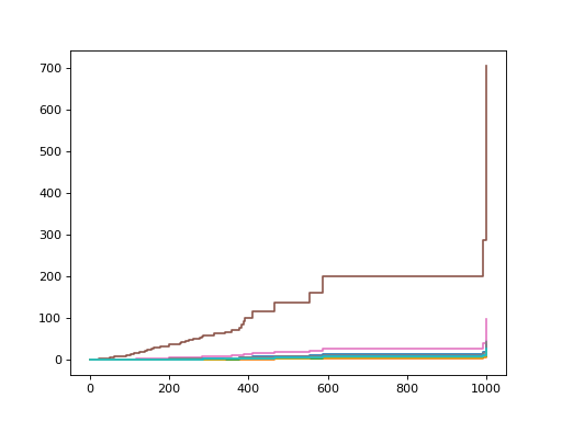
Estimate the cumulative hazard function for the first 10 samples.

>>> chf_funcs = estimator.predict_cumulative_hazard_function(X.iloc[:10])

Plot the estimated cumulative hazard functions.

>>> for fn in chf_funcs:
...     plt.step(fn.x, fn(fn.x), where="post")
...
>>> plt.ylim(0, 1)
>>> plt.show()

predict_survival_function(X, return_array=False)

Predict survival function.

Only available if fit() has been called with loss = “coxph”.

The survival function for an individual with feature vector \(x\) is defined as

\[S(t \mid x) = S_0(t)^{\exp(f(x)} ,\]

where \(f(\cdot)\) is the additive ensemble of base learners, and \(S_0(t)\) is the baseline survival function, estimated by Breslow’s estimator.

Parameters:

• X (array-like, shape = (n_samples, n_features)) – Data matrix.

• return_array (boolean, default: False) – If set, return an array with the probability of survival for each self.unique_times_, otherwise an array of sksurv.functions.StepFunction.

Returns:

survival – If return_array is set, an array with the probability of survival for each self.unique_times_, otherwise an array of length n_samples of sksurv.functions.StepFunction instances will be returned.

Return type:

ndarray

Examples

>>> import matplotlib.pyplot as plt
>>> from sksurv.datasets import load_whas500
>>> from sksurv.ensemble import GradientBoostingSurvivalAnalysis

Load the data.

>>> X, y = load_whas500()
>>> X = X.astype(float)

Fit the model.

>>> estimator = GradientBoostingSurvivalAnalysis(loss="coxph").fit(X, y)

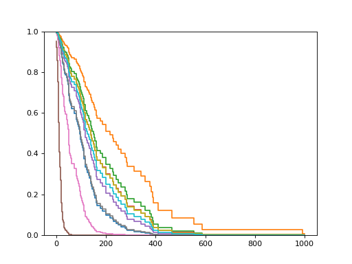
Estimate the survival function for the first 10 samples.

>>> surv_funcs = estimator.predict_survival_function(X.iloc[:10])

Plot the estimated survival functions.

>>> for fn in surv_funcs:
...     plt.step(fn.x, fn(fn.x), where="post")
...
>>> plt.ylim(0, 1)
>>> plt.show()

score(X, y)

Returns the concordance index of the prediction.

Parameters:

• X (array-like, shape = (n_samples, n_features)) – Test samples.

• y (structured array, shape = (n_samples,)) – A structured array containing the binary event indicator as first field, and time of event or time of censoring as second field.

Returns:

cindex – Estimated concordance index.

Return type:

float

set_fit_request(*, monitor: bool | None | str = '$UNCHANGED$', sample_weight: bool | None | str = '$UNCHANGED$') → GradientBoostingSurvivalAnalysis

Request metadata passed to the fit method.

Note that this method is only relevant if enable_metadata_routing=True (see sklearn.set_config()). Please see User Guide on how the routing mechanism works.

The options for each parameter are:

• True: metadata is requested, and passed to fit if provided. The request is ignored if metadata is not provided.

• False: metadata is not requested and the meta-estimator will not pass it to fit.

• None: metadata is not requested, and the meta-estimator will raise an error if the user provides it.

• str: metadata should be passed to the meta-estimator with this given alias instead of the original name.

The default (sklearn.utils.metadata_routing.UNCHANGED) retains the existing request. This allows you to change the request for some parameters and not others.

Added in version 1.3.

Note

This method is only relevant if this estimator is used as a sub-estimator of a meta-estimator, e.g. used inside a Pipeline. Otherwise it has no effect.

Parameters:

• monitor (str, True, False, or None, default=sklearn.utils.metadata_routing.UNCHANGED) – Metadata routing for monitor parameter in fit.

• sample_weight (str, True, False, or None, default=sklearn.utils.metadata_routing.UNCHANGED) – Metadata routing for sample_weight parameter in fit.

Returns:

self – The updated object.

Return type:

object

set_params(**params)

Set the parameters of this estimator.

The method works on simple estimators as well as on nested objects (such as Pipeline). The latter have parameters of the form <component>__<parameter> so that it’s possible to update each component of a nested object.

Parameters:

**params (dict) – Estimator parameters.

Returns:

self – Estimator instance.

Return type:

estimator instance

staged_predict(X)

Predict risk scores at each stage for X.

This method allows monitoring (i.e. determine error on testing set) after each stage.

If loss=’coxph’, predictions can be interpreted as log hazard ratio similar to the linear predictor of a Cox proportional hazards model. If loss=’squared’ or loss=’ipcwls’, predictions are the time to event.

Parameters:

X (array-like, shape = (n_samples, n_features)) – The input samples.

Returns:

y – The predicted value of the input samples.

Return type:

generator of array of shape = (n_samples,)